22 Hash Tables

Modified

March 5, 2026

Note: “Hash Tables” and “P vs. NP” are grouped together in Topic G because it’s convenient for organization, as together they’re about the same size as each other topic. However, they are separate concepts.

Hash tables are a very useful data structure that use randomness to achieve good performance.

Objectives: After learning this material, you should be able to:

Use hash tables as sets, key-value stores, and for similar purposes.
Analyze how hash tables with \(m\) bins and \(n\) items perform under perfect hashing, ideal (random) hashing, and worst-case hashing.
Explain the birthday paradox.

22.1 A hash table as a data structure

Data structures store and retrieve information. A data structure can be broken down into:

An interface: what operations does it support?
An implementation: how do we achieve those operations, and what is the time and space complexity of each?

First, let’s think of a hash table as a Set. It will support these operations:

Operation	Average-case time	Worst-case time	Description
Store(x)	\(O(1)\)	\(O(n)\)	Add x to the set
Get(x)	\(O(1)\)	\(O(n)\)	Check if x is in the set
Remove(x)	\(O(1)\)	\(O(n)\)	Delete x from the set

We will discuss the difference between average-case and worst-case time soon.

It is pretty straightforward to modify such a structure to store key-value pairs; such a data structure is often called a table, a dictionary, or a map. If we want to store a key \(k\) associated to a value \(v\), then we simply treat \(k\) as we did \(x\) above, and when we go to store it in the data structure, we also store \(v\) along with it. Then, when we want to look up \(k\), we can find it and also retrieve \(v\).

Operation	Average-case time	Worst-case time	Description
Store(k,v)	\(O(1)\)	\(O(n)\)	Store key-value pair \(k,v\)
Get(k)	\(O(1)\)	\(O(n)\)	Retrieve value \(v\) for key \(k\), if any
Remove(k)	\(O(1)\)	\(O(n)\)	Delete \(k\) and its value

One can also use a binary tree or other data structures to implement these operations, but not as quickly (in the average case).

An example use case would be counting the number of times each word appears in a document:

Algorithm 22.1

count_words(document):
   hash_table = new hash table
   for each word in document:
      previous_count = hash_table.Get(word)  # or zero if not yet stored
      new_count = previous_count + 1
      hash_table.Store(word, new_count)

22.2 Implementing hash tables

In general, we will implement a hash table by using an array to store the items. If we have \(n\) items, we would like to have an array of length \(m=n\), so that there is one slot per item.

To store the items, we will choose in advance a hash function that assigns each item a location in the array.

Definition 22.1 (Hash function) Given a universe \(U\) of items and an array length \(m\), a hash function is a function \(h: U \to \{1,\dots,m\}\) that assigns each item a location in the array.

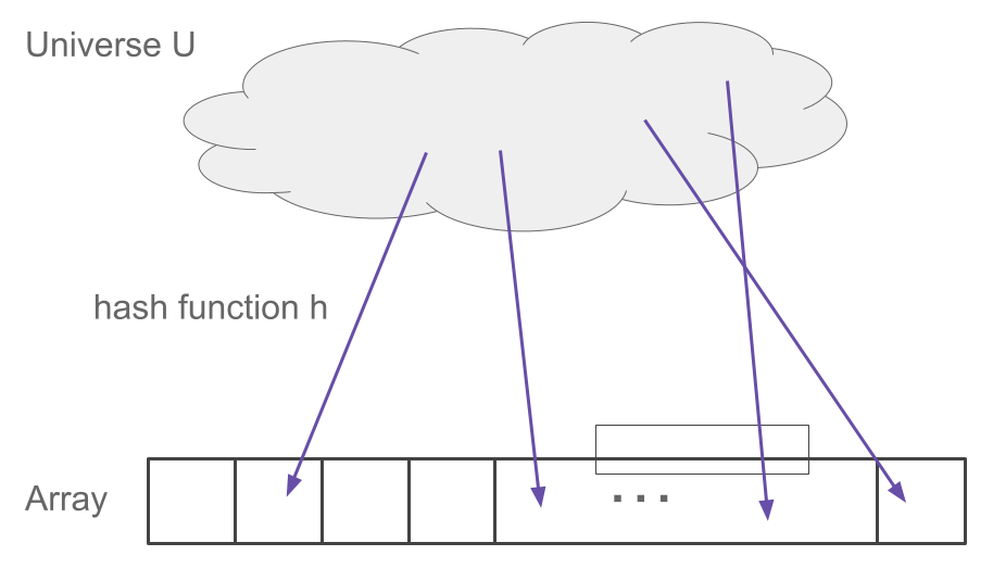
Visual depiction of a hash function mapping items in a universe to an array.

However, the problem is that usually, there is a large “universe” of items that might arrive, much larger than \(n\). For example, we may be storing 64-bit integers in a set. In this case, there are \(2^{64}\) possible integers that might arrive. Even if only a small number of them do, we don’t know in advance which ones.

Exercise 22.1 Suppose we are hashing 64-bit integers to \(\{0,\dots,1023\}\). We will use a naive hash function, h(x) = x % 1024, where % is the “modulo” operator.

Part a. Give a set of \(1024\) integers that are “perfectly hashed”: each one goes to a different location. Briefly explain.

Part b. Give a set of \(1024\) integers that are hashed in the worst way: they all go to the same location. Briefly explain.

Sample solution.

Part a. For example, we can take \(\{0,1,\dots,1023\}\). Each number is hashed to itself.

Part b. For example, \(\{1, 1025, 2049, \dots\}\), that is, the numbers of the form \(1024k + 1\) for \(k = 0, \dots, 1023\). All of these are hashed to slot 1.

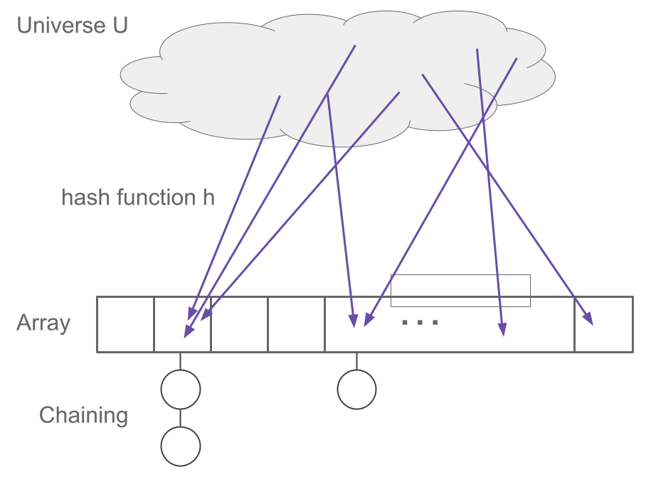
22.2.1 Collisions and chaining

If two items are hashed to the same location, we call this a collision. Every hash table needs a strategy to handle collisions. We will focus on a straightforward strategy called chaining. In chaining, we simply make a list (such as a linked list) for each array location. If multiple items arrive, we add them to the list for that location.

Visual depiction of chaining as as list of items attached to an array slot.

Note 1 Hash table implementation.

To summarize, the hash table is implemented as follows. Before starting, we pick a hash function h. We will discuss the choice of h later.

Store(x):

Let j = h(x).
If there is no item at location j, put x there.
If there are already items there, add x to the linked list for location j.

Get(x):

Let j = h(x).
If there is no item at location j, return None.
If there is one or more items, look through the linked list for x and return whether you found it.

Remove(x):

Follow the instructions for Get(x), but if you find x, delete it from the list.

22.3 Analysis of hash tables

Suppose we will Store() \(n\) items total in a hash table with array length \(n\). Then, we will make \(n\) calls to Get(). What will be the total time complexity?

Note 2 We will assume that all of our hash functions run in constant time, \(O(1)\), per call.

In the best case, each item is hashed to a different location. Because all of the lists are of length \(1\), all of the store and retrieve operations run in constant time. Therefore, the total time is \(O(n)\), and each Store() and Get() command runs in \(O(1)\) time.

In the worst case, all of the items are hashed to the same location. The time for all of the Store and Get commands is \(O(1 + 2 + \cdots + n) = O(n^2)\). Therefore, on average, each Store() and each Get() command runs in \(O(n)\) time.

Now, let’s consider the average case. To do so, we have to see what hash function we will actually use. We will use randomness to try to “spread out” the hash function’s outputs. For analysis, we’ll make this assumption.

#Ideal hash function An ideal hash function is one where each item’s location is chosen uniformly at random and independently from \(\{1,\dots,m\}\).

Assuming an ideal hash function, each bin has on average one element. Therefore in the average case, each Store() command and each Get() command use O(1) operations. (To be more formal, one can show that the sum over all \(n\) Store() and Get() commands is \(O(n)\), which gives \(O(1)\) per command average-case.)

Remark 22.1. Using an ideal hash function is modeled by the “balls in bins” problem where we throw \(n\) balls (these are the items being hashed) into \(m\) bins (the array locations), where each ball lands in a independent, uniformly randomly chosen bin.

Exercise 22.2 Suppose we throw \(n\) balls into \(n\) bins, i.e. we hash \(n\) items into \(n\) array slots using an ideal hash function. What is the probability that bin number 1 is empty (has no items)?

Solution.

Each ball misses bin 1 with probability \(1 - \frac{1}{n}\). Since they’re independent, the probability they all miss is \(\prod_{j=1}^n (1 - \frac{1}{n}) = (1 - \frac{1}{n})^n \to \frac{1}{e}\) as \(n \to \infty\). So the probability is about \(\frac{1}{e} \approx 0.3678\).

Note 3

23 Implementation

To recap, we hope to have a hash function that is as close to “ideal” as possible. In practice, there are many hash functions, and they often do have a randomly chosen component. They often work by using arithmetic operations on the bits of the input in order to “scramble” them and produce a randomly-distributed output.

Another implementation note is that, often, we don’t know in advance how many items we’ll store in the hash table. This can be addressed by starting with a small table and doubling the size of the table once the number of items grows large enough, reassigning all items to the new array slots. We repeat as needed.

23.1 Birthday paradox

When analyzing hash tables, one question is how many collisions will occur and when they will occur. Let’s start by asking when the first collision will occur. How many balls do we need to throw into \(n\) bins before we expect that two balls have landed in the same bin?

Proposition 23.1 If we throw \(k\) balls into \(n\) bins, the expected number of collisions is \({k \choose 2} \frac{1}{n} = \frac{k(k-1)}{2n}\).

Proof. Consider any pair of balls. What is the probability they land in the same bin? The answer is \(\frac{1}{n}\): the first ball lands in some bin, and the second ball has a \(\frac{1}{n}\) chance of landing in that bin.

But now the expected number of collisions is just the sum, over all pairs of balls, of the probability that pair collides. There are \({k \choose 2} = \frac{k(k-1)}{2}\) pairs of balls, so the answer is \({k \choose 2}\frac{1}{n}\).

Corollary 23.1 For \(k \approx \sqrt{2n}\), after throwing \(k\) balls, there is in expectation one collision.

This result is surprising because \(\sqrt{2n}\) is much less than \(n\); we probably get a collision very quickly! An example is the “birthday paradox”. There are about 365 days in a year. If we pretend that each person’s birthday is chosen independently and uniformly at random, then how many people do we need in a room before we expect that some pair share a birthday? The answer is only about \(27 = \sqrt{2 \cdot 365}\).

This result implies that we need a strategy for handling collisions even when the number of items is much smaller than the size of the array.