12  Minimum Spanning Trees

This section discusses a fundamental problem in graph theory and uses greedy algorithms to solve it.

Objectives. After learning this material, you should be able to:

• Define the minimum spanning tree (MST) problem.
• Use properties of spanning trees to solve related problems.
• Execute Prim’s and Kruskal’s algorithms.

12.1 Spanning trees

First, we need to recall the definition of a tree. Previously in this class, we defined rooted trees. We can think of a tree as a rooted tree, where we deleted all information about which node is the root and which nodes are children of which. Here is a formal definition:

Definition 12.1 (Tree) An undirected graph \(T = (V,E)\) is a tree if it is connected and has no simple cycles.

Remember that connected means there is a path from every vertex to every other vertex. A simple cycle is a path of length at least three that starts and ends at the same vertex and does not repeat edges. Here is a nice fact about trees.

Proposition 12.1 Any tree on \(n\) vertices has exactly \(n-1\) edges.

Proof. By induction on \(n\). The base case is \(n=1\). A graph with one vertex will have no edges (we generally assume that self-loops are not allowed), so the formula is satisfied.

Now let \(n \geq 2\) and suppose that any tree on \(n' < n\) vertices has exactly \(n'-1\) edges. Consider a tree on \(n\) vertices. Let us delete any edge \(\{u,v\}\). We first claim this disconnects the graph into two disjoint trees. First, deleting an edge cannot have created a cycle. Next, it is partitioned into two connected components: originally, every vertex was reachable from \(u\), and the path from \(u\) either included the edge \(\{u,v\}\) or not. If so, the vertex is still reachable from \(v\) after the disconnection, and if not, it is still reachable from \(u\) after the disconnection. Further every vertex is in either one case or the other, but not both, as otherwise there would be a cycle in the original graph involving a path to the vertex from \(u\) and from \(v\), along with the edge \(\{u,v\}\). So the graph is partitioned into two disjoint connected acyclic graphs, i.e. trees.

The trees have \(n_1,n_2 \geq 1\) vertices with \(n_1 + n_2 = n\). By inductive hypothesis, they have \(n_1-1\) and \(n_2-1\) edges. Adding \(\{u,v\}\), the total number of edges in our original tree is \(n_1 - 1 + n_2 - 1 + 1 = n-1\).

Next, we can define a spanning tree. Intuitively, given a connected, undirected graph, we may want to delete as many edges as possible while keeping the graph connected. The minimum set of edges we need to keep form a tree, called a spanning tree.

Definition 12.2 (Spanning tree) In an undirected graph \(G = (V,E)\), a spanning tree is a tree \(T = (V,E')\) where \(E' \subset E\). In other words, it is a subgraph of the original graph that includes all the vertices and is a tree.

Exercise 12.1 Give a spanning tree of this graph.

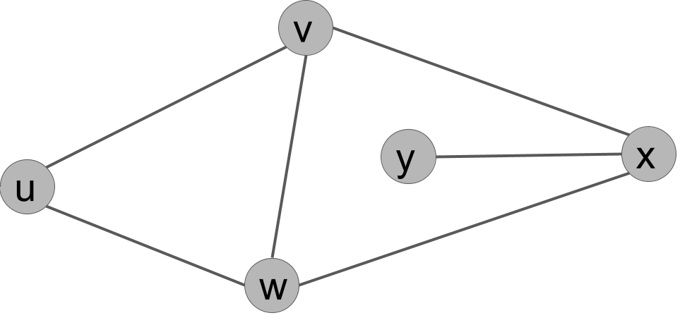
Example solution.

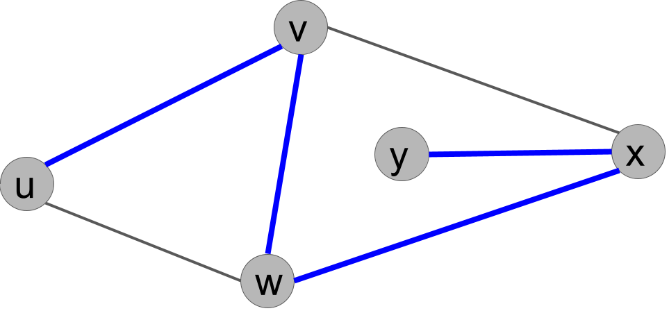
There are several solutions. Because there are 5 vertices, any subset of 4 edges that keep the graph connected form a spanning tree. Here is one (the thick blue edges):

12.2 Minimum spanning tree (MST) and reverse-deletion

In the minimum spanning tree problem, our graph is undirected and weighted. We assume the weight \(wt(u,v)\) on each edge is positive.

Minimum spanning tree (MST) problem:

• Input: a connected, weighted, undirected graph. We assume for simplicity that all edge weights are distinct.
• Output: a spanning tree where the sum of the edge weights is as small as possible.

This problem can arise in many contexts. Picture a communication network, such as a network of computers. We want to ensure that the network is connected so that every node can send a message through the network to every other node. However, maintaining all of the links (edges) may be costly. We want to reduce the number of links to the minimum-cost set needed in order to maintain communication.

Exercise 12.2 Give a minimum spanning tree of this graph.

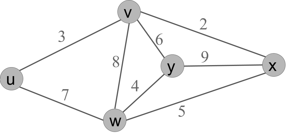
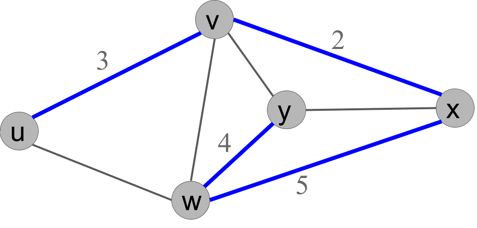
Solution.

There is only one minimum spanning tree, shown here in blue. Its total weight is 2+3+4+5 = 14.

12.2.1 The Reverse-Deletion Algorithm

It is worth noting the following point. Can you prove it?

Observation 1 The minimum-cost set of edges that keep the graph connected will always form a tree.

Proof.

Suppose we have a set of edges where the graph is connected, but not a tree. Then there is a cycle. If we delete one edge \(\{u,v\}\) from the cycle, the graph is still connected, because we can still get from every node on the cycle to every other node. And deleting the edge has reduced the total cost of this set of edges. We can repeat this argument as long as the graph has cycles until we end with a connected, acyclic graph: a tree.

This observations gives an idea for our first greedy algorithm for MST.

The Reverse-Deletion Algorithm:

• Sort the edges from largest weight to smallest.
• Go through the list, deleting each edge unless doing so disconnects the graph.

For correctness, as with Dijkstra’s algorithm, we need a key fact about the problem. Here is the fact:

Proposition 12.2 For any simple cycle in the graph, the maximum-weight edge in the cycle is not part of any minimum spanning tree.

Proof. Let \(v_1,\dots,v_k=v_1\) be a simple cycle and suppose without loss of generality that \(\{v_1,v_2\}\) is the maximum-weight edge in the cycle. Suppose we have a spanning tree \(T\) containing \(\{v_1,v_2\}\). We prove it is not a minimum spanning tree.

Delete \(\{v_1,v_2\}\) from the tree, leaving us with two disjoint trees, say \(T_1\) containing \(v_1\) and \(T_2\) containing \(v_2\). Adding any edge between a vertex in \(T_1\) and a vertex in \(T_2\) will connect the trees into a spanning tree again. And in the original graph, there is a path \(v_2,\dots,v_{k-1},v_1\). Since the start is in \(T_2\) and the end is in \(T_1\), at least one of these edges crosses over. And it must have smaller weight than \(\{v_1,v_2\}\), so adding it results in a spanning tree with smaller weight than \(T\), so \(T\) could not have been a MST.

Theorem 12.1 The Reverse-Deletion algorithm correctly produces a MST.

Proof. Suppose that deleting an edge does not disconnect the graph. Then that edge must have been part of a simple cycle, because there is still a path between its endpoints. So by the Proposition, that edge cannot have been part of any minimum spanning tree. Therefore, if we delete it, a minimum spanning tree of the resulting graph is also a MST of the original graph. Now we just need to note that Reverse Deletion continues until the set of remaining edges is a spanning tree, because otherwise, by definition, there is a cycle and some edge could be deleted. Since it stops at a spanning tree, that spanning tree is a MST of the original graph.

12.3 Kruskal’s and Prim’s algorithms

We will look at two other correct greedy algorithms for minimum spanning tree. They both rely on the following key fact.

Proposition 12.3 Let \(R,S\) be any cut in the graph, meaning a partition of the graph into two disjoint sets of vertices. Let \(\{u,v\}\) be the minimum-cost edge that crosses the cut. Then every MST of the graph contains \(\{u,v\}\).

Proof. Consider any spanning tree of the graph that does not contain \(e\). We will show it is not a minimum spanning tree.

Suppose without loss of generality that \(u \in R\) and \(v \in S\). Because it’s connected, there is a path in the spanning tree from \(u\) to \(v\). This path “crosses” the cut at some point, i.e. includes some edge \(\{u',v'\}\) with \(u' \in R\) and \(v' \in S\). Let us delete \(\{u',v'\}\) and add \(\{u,v\}\). By assumption, the total cost of the edges has decreased. Is it still a spanning tree? It is still connected, because there is now a path from \(u'\) back to you, across \(\{u,v\}\) to \(v\), and then to \(v'\). So any prior path that used \(\{u',v'\}\) can be transformed into a path that uses \(\{u,v\}\). Similarly, there are no cycles, because if there is a cycle including \(\{u,v\}\) now, we could transform it into a cycle that uses \(\{u',v'\}\) in the original graph. (The cycle might not be simple, but we can turn it into a simple cycle from there.)

This fact suggests an algorithm that is a sort of mirror to the Reverse Deletion algorithm.

Kruskal’s algorithm:

• Sort the edges from smallest weight to largest.
• Go through the list, adding each edge to the graph unless doing so creates a cycle.

Theorem 12.2 Kruskal’s algorithm outputs a minimum spanning tree.

Proof. When we add an edge \(\{u,v\}\), let \(R\) be the set of vertices reachable from \(u\) along edges added so far, and let \(S\) be the remaining vertices. Note that adding any edge that crosses the cut would not create a cycle, since currently no edges cross the cut. Therefore, \(\{u,v\}\) must be the minimum-weight edge that crosses this cut, since we are adding edges in order. So by the Proposition, every minimum spanning tree contains \(\{u,v\}\), so we are safe to add it to our solution. Now we just need to show that Kruskal’s produces a spanning tree. The output doesn’t have cycles by definition. But it is a tree, since if it were disconnected at the end, there would be some edge that could have been added (as the original graph was connected), a contradiction. So Kruskal’s produces a spanning tree, and it is minimum because it only contains edges that are in every MST.

A small complaint about Reverse-Deletion and Kruskal’s is that they are not very efficient, at least if implemented in a straightforward way. First, sorting the edges at the beginning takes \(O(m \log(m))\) time, and \(m\) can be quite a bit larger than \(n\). Second, checking in every loop for whether a cycle has been created takes a significant amount of time. A straightforward approach is to use BFS or DFS each time to check for a cycle. However, doing this every loop is a somewhat slow process. (For Kruskal’s, the time complexity can be improved significantly with the union-find data structure, but we won’t cover that here.)

Can we do better? Yes: here is Prim’s algorithm.

Prim’s algorithm:

• Pick any vertex \(u\), and add it to our set \(R\).
• Add the minimum-cost edge \(\{u,v\}\) attached to \(u\) to our solution, and add its other endpoint \(v\) to \(R\).
• Continuing, add the minimum-cost edge leaving \(R\) to our solution and add its other endpoint to \(R\).
• Stop when \(R = V\), the set of all vertices.

Theorem 12.3 Prim’s algorithm outputs a minimum spanning tree.

Proof. At every step, we add the minimum-cost edge that crosses a cut in the graph, where the cut is \(R\) and \(V \setminus R\). So by the Proposition, every edge we add must be part of every minimum spanning tree. And we certainly produce a spanning tree, because we never create a cycle and we eventually connect all vertices.

12.3.1 Running time analysis of Prim’s algorithm

To analyze running time, we should have a more precise definition of the algorithm. In fact, it will look extremely similar to Dijkstra’s algorithm. As with Dijkstra’s, we will use a Priority Queue.

Algorithm 12.1 (Prim’s algorithm)  

prim(G):
   # G = (V,E) is a weighted, undirected, connected graph
   Q = new Priority Queue
   for all vertices u:
      best_weight[u] = infinity
      best_edge[u] = null
      marked[u] = false
      Q.insert(u, infinity)
   let s be any vertex of G
   Q.update(s, 0)
   let F = empty list       # edges of the spanning tree
   while Q.size() > 0:
      u = Q.pop_smallest()
      marked[u] = true
      F.add(best_edge[u])   # does nothing if best_edge[u] is null
      for v in N(u):
         if not marked[v] and wt(u,v) < best_weight[v]:
            best_weight[v] = wt(u,v)
            best_edge[v] == {u,v}
            Q.update(v, wt(u,v))
   return (V, F)

To understand the pseudocode, see if you can answer this question (you will want to take another look at Dijkstra’s).

Exercise 12.3 What is the key difference between Prim’s and Dijktra’s algorithms? How do these differences result in one solving MST while the other solves shortest paths?

Solution.

The key difference is that Dijkstra’s tracks the smallest total distance from the source to a given vertex. Prim’s tracks the smallest edge to the vertex from any previously-visited vertex. This means that Dijkstra keeps popping vertices with smallest distance from the source, but Prim keeps popping vertices that have the smallest edge to the current connected component. So Dijkstra is finding paths from \(s\) that are as short as possible, while Prim is connecting a tree as cheaply as possible.

The running time of this implementation is essentially identical to Dijksta’s. If we use a Fibonacci heap, we obatin the following analysis, which is the same as in Dijkstra’s.

Operations	Total time with F. heap
\(O(n)\) calls to Q.insert()	\(O(n)\)
\(O(n)\) calls to Q.pop_smallest()	\(O(n \log(n))\)
\(O(m)\) calls to Q.update()	\(O(m)\)

The result is a running time of \(O(m + n \log(n))\), just as with Dijkstra’s algorithm. We also should note that we have \(O(n + m)\) operations otherwise, but this will be dominated in big-O by the complexity of the heap operations.