9 Shortest Paths
We now turn to one of the most important graph problems, finding shortest paths through a graph.
Objectives. After learning this material, you should be able to:
- Execute BFS and Dijkstra’s algorithm to find shortest paths in a graph.
- Show how BFS and Dijkstra’s fail when their assumptions are not satisfied.
- Discuss the runtime analysis of Dijkstra’s depending on the priority queue data structure.
9.1 The shortest paths problem
So far, we have used DFS and BFS to explore the structure of a graph without a particular destination in mind. Now, we’ll consider the shortest paths problem. This problem needs to be solved every time you search for directions (driving, walking, etc.), as well as in many other cases.
Shortest paths problem.
- Input: a graph \(G = (V,E)\) and a start vertex \(s \in V\).
- Output: an array
distwhere, for each \(t \in V\),dist[v]is the length of the shortest path from \(s\) to \(t\).
This is often called the single-source shortest paths problem because, given a single source \(s\), we find the shortest paths to all possible destinations \(t\). Often, we only want to know the distance from \(s\) to one particular destination \(t\), but the algorithms will turn out to be almost the same.
9.2 Unweighted graphs
First, we will consider unweighted graphs. Here the length of a path is the number of edges or “hops”. We will modify BFS to solve this problem. In this variant, dist[v] represents the distance to v. We can also use it in the same way as the marked array from the previous BFS implementation. If dist[v] == infinity, then v is not yet marked. If dist[v] is a number, then v has been marked.
Algorithm 9.1 (BFS for Shortest Paths)
BFS_dist(G, s):
   # G = (V,E) is an unweighted graph and s a vertex
   for each v in V:
      let dist[v] = infinity
   let Q = new FIFO_Queue
   set dist[s] = 0
   Q.append(s)
   while Q.size() > 0:
      let v = Q.pop()
      for each neighbor w of v:
         if dist[w] = infinity:   # not yet marked
            Q.append(w)
            set dist[w] = dist[v] + 1
   return dist
As an exercise, you can go back to the previous example graph, or draw a new one, and practice executing BFS_dist.
9.2.1 Correctness
Theorem 9.1 BFS_dist(G,s) correctly solves the shortest-paths problem on unweighted graphs.
Proof. One note is that, once a node’s distance is set to a number, it is never updated. This follows because we only set a node’s distance if it is currently infinity.
We proceed inductively. The claim we will prove is that we pop nodes from the queue in order of distance: all nodes at distance 0, all nodes at distance 1, and so on; and when we set a node’s distance, it is correct.
The base case is \(d=0\). The only distance-zero node is the start node, s. The algorithm does set dist[s] = 0 in line 6, then pop it from the queue first.
Inductively, suppose the claim is true up to distance \(d\) for some \(d \geq 0\). We must prove it for distance \(d+1\). A node w is at distance \(d+1\) if there is a path \(s,\dots,w\) of distance \(d+1\), but there is no path of distance \(d\) or shorter. Because there’s no path of distance \(d\) or shorter, by IH, we pop and set all the nodes up to distance \(d\) before we get to any node of distance \(d+1\). But a node is at distance \(d+1\) if it is a neighbor of a node at distance \(d\). By IH, we have just popped all nodes of distance \(d\) and set the distances for all their unmarked neighbors to distance \(d+1\). That proves the inductive claim.
To finish, we should note that if there is no path at all from \(s\) to \(v\), then at the end, we have dist[v] = infinity, which correctly indicates that there is no path.
9.2.2 Time and space complexity
By checking the small changes we made from BFS to BFS_dist, we can confirm that the time complexity is still \(O(n + m)\). It’s also good to check the space usage. We have several variables representing nodes, which take \(O(1)\) space. Then we have dist, and array of length \(n\). Then we have Q. We have noted that every node is added to Q at most once, so it requires at most \(n\) space as well. We conclude that the algorithm uses \(O(n)\) space. (Note that the input, an adjacency list, would take more space than this, \(O(n + m)\).)
9.2.3 Finding the paths themselves
An important point is that BFS_dist found the lengths of the shortest paths, but it didn’t actually find the paths themselves! It could tell us that a certain node had distance \(103\) from \(s\), but not how to get there in \(103\) steps. However, this can be easily fixed. When we set dist[w] = dist[v] + 1, we simply add a note at \(w\) to say that the shortest way to get there is from \(v\). And \(v\) will have its own note, and so forth. Here’s the implementation; the two new lines are 5 and 16.
Algorithm 9.2 (BFS with Path Pointers)
BFS_dist(G, s):
# G = (V,E) is an unweighted graph and s a vertex
for each v in V:
let dist[v] = infinity
let prev[v] = null
let Q = new FIFO_Queue
set dist[s] = 0
Q.append(s)
while Q.size() > 0:
let v = Q.pop()
for each neighbor w of v:
if dist[w] = infinity:
Q.append(w)
set dist[w] = dist[v] + 1
set prev[w] = v
return dist, prev
get_path(s, t, prev):
path = [t] # list with just t
while t != s:
set t = prev[t]
if t == null:
return "no path exists"
put t at front of path
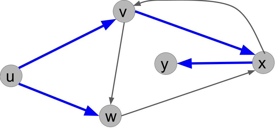
return path For an example, we can revisit our example graph Figure 8.4 with source \(u\) (also shown below in Figure 9.1). Here, prev will point in the opposite direction of the blue arrows. For instance, the shortest path from \(u\) to \(y\) has length 3. When we call get_path(u, y, prev), it follows these steps:
- We first put \(y\) in our list, called
path. - Then we get
x = prev[y]. We put \(x\) at the front of our list, which is nowpath = [x,y]. - Then we get
v = prev[x]. We put \(v\) at the front of our list, which is now[v,x,y]. - Then we get
s = prev[v]. We put \(s\) at the front of our list, which is now[s,v,x,y]. - Then we terminate the loop and return our list,
path = [s,v,x,y].
9.3 Weighted graphs
We’ll now consider graphs with weights on the edges. As mentioned above, the length of a path is now the sum of the weights of the edges in the path.
9.3.1 Failure of BFS on weighted graphs
Does BFS find shortest paths on weighted graphs? We know it probably shouldn’t, because it doesn’t look at the edge weights at all. But how can it fail? You should try to solve the following exercise. A solution is not provided, because this is a problem every student needs to be able to do!
Exercise 9.1 Give a weighted graph G, source s, and destination t for which BFS(G,s) does not find the shortest path from s to t.
Hint.
BFS will always find the smallest number of hops from s to t. What if there is a path with more hops, but shorter distance?
9.3.2 Dijkstra’s algorithm
We’ll now solve the problem for weighted graphs. Let \(wt(u,v)\) be the weight of the edge from u to v. We assume the weights are positive, i.e. \(wt(u,v) > 0\) for all \(u,v\). We can let \(wt(u,v) = \infty\) to denote that there is no edge between \(u\) and \(v\).
9.3.2.1 The key fact
To create an algorithm, usually, we need a fact. The fact about how the problem is structured allows us to write an algorithm that leverages the structure. With BFS, a key fact we used was that if v is at distance \(d+1\), then there is a vertex \(u\) at distance \(d\) and an edge \((u,v)\). Our key fact for weighted graphs is similar.
Fact 1 On a weighted graph \(G\) with source vertex s, let \(d(v)\) be a function denoting the length of the shortest path from s to v. Let \(IN(v)\) be the set of in-neighbors of \(v\), i.e. the vertices that have an edge to \(v\). Then for any \(v \neq s\):
- For all \(u \in IN(v)\), we have \(d(v) \leq d(u) + wt(u,v)\).
- Furthermore, \(d(v) = \min_{u \in IN(v)} d(u) + wt(u,v)\).
The fact is saying that the shortest path to v has to go from s to one of v’s in-neighbors, then hop to v. Furthermore, the shortest path to v has to take the shortest path to one of its in-neighbors, then hop to v. This fact is illustrated in the next figure, where other edges of the graph are omitted and the dashed lines represent some shortest path through the graph.
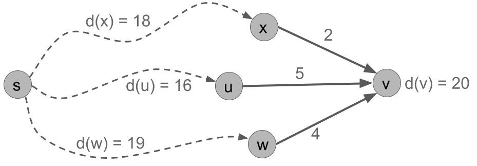
For vertex v, we can check the two points of Fact 1 in the following table. We see that the distance to v is d(v) = 20, which is the minimum over these options.
| d(x) = 18 | wt(x,v) = 2 | d(x) + wt(x,v) = 20 |
| d(u) = 16 | wt(x,v) = 5 | d(x) + wt(x,v) = 21 |
| d(x) = 19 | wt(x,v) = 4 | d(x) + wt(x,v) = 23 |
9.3.2.2 Dijkstra’s
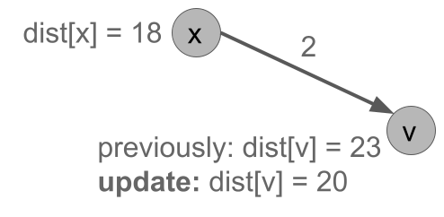
The idea of Dijkstra’s algorithm is similar to a modified breadth-first search. We will process vertices in order of their distance from the source. For each vertex, we will set the distances of its neighbors. However, instead of locking in the distance the first time, we will update the distance using the idea of the fact.
The other change is that we need a fancier data structure, which we call a priority queue. In a priority queue, every object in the queue has a value. We always pop the object with the smallest value. Here are the operations; we’ll discuss the time complexity later.
Priority Queue:
| Operation | Meaning |
|---|---|
| insert\((u, d)\) | insert object \(u\) with value \(d\) |
| update\((u, d)\) | update the value of \(u\) to be \(d\) |
| pop_smallest() | remove and return the object with smallest value |
| size() | return the number of objects in the queue |
Now, we can give Dijkstra’s algorithm.
Algorithm 9.3 (Dijkstra’s)
dijkstra(G, s):
   # G is a weighted graph with weights w(u,v)
   let Q = new Priority_Queue
   for all vertices u:
      let dist[u] = infinity
      Q.insert(u, infinity)
   set dist[s] = 0
   Q.update(s, 0)
   while Q.size() > 0:
      let u = Q.pop_smallest()
      for each neighbor v of u:
         set dist[v] = min(dist[v], dist[u] + w(u,v))
         Q.update(v, dist[v])
   return dist
As we mentioned, there are two main changes from BFS. The first is to use a priority queue so that we always pop the remaining vertex with minimum distance. The second is that when we process u, we update the distances of all its neighbors v. If dist[v] is currently larger than the distance available by going to u and then hopping to v, we update it.
dijkstra(G,s).
As usual with algorithms, the best way to understand it is to execute it by hand on some examples.
Exercise 9.2 Given the below graph, simulate the execution of Dijkstra’s algorithm starting from u. Report, at the beginning of each iteration of the while loop, the state of the priority queue and the distance table, and which vertex is popped from the queue.
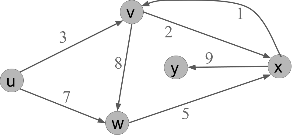
Example solution.
| Round | dist[u] | dist[v] | dist[w] | dist[x] | dist[y] | queue | vertex popped |
|---|---|---|---|---|---|---|---|
| 1 | 0 | \(\infty\) | \(\infty\) | \(\infty\) | \(\infty\) | u, v, w, x, y | u |
| 2 | 0 | 3 | 7 | \(\infty\) | \(\infty\) | v, w, x, y | v |
| 3 | 0 | 3 | 7 | 5 | \(\infty\) | x, w, y | x |
| 4 | 0 | 3 | 7 | 5 | 14 | w, y | w |
| 5 | 0 | 3 | 7 | 5 | 14 | y | y |
| 6 | 0 | 3 | 7 | 5 | 14 | \(\quad\) |
9.3.3 Reconstructing the actual paths
Just as with BFS, the initial version of Dijkstra presented only returns the length of the shortest path, not the path itself. But just as with BFS, it is pretty straightforward to modify the algorithm in the same way: we maintain a prev array, where prev[v] represents the previous vertex for \(v\) along the shortest path from \(s\). Here is how we update the algorithm, in lines 7 and 15-16.
Algorithm 9.4
dijkstra(G, s):
   # G is a weighted graph with weights w(u,v)
   let Q = new Priority_Queue
   for all vertices u:
      let dist[u] = infinity
      Q.insert(u, infinity)
      let prev[u] = null
   set dist[s] = 0
   Q.update(s, 0)
   while Q.size() > 0:
      let u = Q.pop_smallest()
      for each neighbor v of u:
         set dist[v] = min(dist[v], dist[u] + wt(u,v))
         Q.update(v, dist[v])
         if dist[v] == dist[u] + wt(u,v):
            set prev[v] = u
   return dist, prev
In particular, in lines 15-16, if the current shortest path to v is indeed from u, then we set prev[v] = u. Given these changes, reconstructing a shortest path can be done with the same algorithm get_path(s, t, prev), from BFS (alg. 9.2).
9.3.4 Correctness
Theorem 9.2 For graphs with positive edge weights, Dijkstra’s algorithm correctly solves the single-source shortest paths problem.
Proof. Let us number the vertices in order that the algorithm pops them from the queue: \(s=v_1,v_2,v_3,\dots,v_n\).
We prove by induction on \(k=1,\dots,n\) that, when we pop \(v_k\), its distance is set correctly: dist[v_k] \(= d(v_k)\). We note that distances start at \(\infty\) and only decrease, and cannot fall below the true distances because every update corresponds to the distance of a path to \(v_k\). So if dist[v] \(= d(v)\) at any point, the equality holds true forever.
Base case: \(k=1\), i.e. the case of \(s\). When we pop \(s\), we correctly have dist[s] = 0.
Inductive case: Suppose that \(v_1,\dots,v_k\) had their distances set correctly when popped. We first note that for all remaining \(v\), we have dist[v] equal to the shortest path of the form \(s,\dots,u,v\) where all of \(s,\dots,u\) have already been popped. This follows because when each in-neighbor \(u\) of \(v\) was popped, its distance was set correctly by inductive hypothesis and dist[v] = min(dist[v], dist[u] + wt(u,v)) was called.
Now consider the shortest path that is not of this form. It must be of the form \(s,\dots,u,v',\dots,v\) where \(s,\dots,u\) have been popped, but \(v'\) has not. Because \(v\) was the smallest object in the priority queue, we must have dist[v] <= dist[v']. But by the note above, since this path starts \(s,\dots,u\), if it is a shortest path, it would have dist[v'] = d(v'). So the distance to \(v\) along this path, which is only longer, is longer than dist[v]. So this path is longer. So dist[v] is indeed equal to the shortest distance from \(s\).
9.3.5 Running time
First, let’s analyze Dijkstra for a generic priority queue. Then, we’ll plug in specific implementations of the queue. This time, we’ll skip any \(O(1)\) time operations and just look at how many times each loop runs.
dijkstra(G, s):
   # G is a weighted graph with weights w(u,v)
   let Q = new Priority_Queue
   for all vertices u:                       # n iterations
      let dist[u] = infinity for all u in V
      Q.insert(u, infinity)
   set dist[s] = 0
   Q.update(s, 0)
   while Q.size() > 0:                       # at most n iterations
      let u = Q.pop_smallest()
      for each neighbor v of u:              # at most O(n + m) iterations total
         let dist[v] = min(dist[v], dist[u] + wt(u,v))
         Q.update(v, dist[v])
   return dist
The time complexity is therefore \(O(n+m)\) plus the time for \(O(n)\) calls to Q.insert() and Q.pop_smallest() + \(O(n + m)\) calls to Q.update(). To complete the analysis, we need to know the total time taken by these priority queue operations.
9.3.5.1 A binary tree priority queue
One way to implement a priority queue is with a binary search tree, which keeps its objects sorted by value. In a binary search tree, all operations take \(O(\log(n))\) time, where the maximum number of vertices in the tree is \(n\).
Binary tree:
| Operation | Time complexity | Meaning |
|---|---|---|
| insert\((u, d)\) | \(O(\log n)\) | insert object \(u\) with value \(d\) |
| update\((u, d)\) | \(O(\log n)\) | update the value of \(u\) to be \(d\) |
| pop_smallest() | \(O(\log n)\) | remove and return the object with smallest value |
| size() | \(O(1)\) | return the number of objects in the queue |
In this case, our running time is:
\(O(n + m + n \log(n) + (n + m)\log(n)) = O((n + m)\log(n))\).
However, there are slightly faster data structures available. The best for Dijkstra’s is the Fibonacci heap. It has the amazing property that, over the course of all \(n\) insertions and updates, the total time taken is \(O(n)\). This is a slightly different statement than saying that the running time is \(O(1)\) per update, because there could be a few updates that are slower than that. Hence, we call this kind of guarantee an \(O(1)\) “amortized” per operation.
Fibonacci heap:
| Operation | Time complexity | Meaning |
|---|---|---|
| insert\((u, d)\) | \(O(1)\) amortized | insert object \(u\) with value \(d\) |
| update\((u, d)\) | \(O(1)\) amortized | update the value of \(u\) to be \(d\) |
| pop_smallest() | \(O(\log n)\) | remove and return the object with smallest value |
| size() | \(O(1)\) | return the number of objects in the queue |
With this data structure, our running time is:
\(O(n + m + n \log(n) + (n + m) \cdot 1) = O(n \log(n) + m)\).
Recall that, for unweighted graphs, BFS ran in time \(O(n + m)\). Dijkstra’s runs in time \(O(n \log(n) + m)\), just slightly slower while handling any positive edge weights.