8  Exploring Graphs

In this section, we’ll learn about algorithms for exploring graphs by hopping from vertex to neighboring vertex.

Objectives. After learning this material, you should be able to:

• Describe search trees produced by exploring a graph.
• Execute depth-first search and breadth-first search on a graph and recall their runtime analyses.
• Contrast the search trees that can be produced by DFS versus by BFS.

8.1 Depth-first search

One of the most basic and important tasks to do on graphs is to explore them: starting from a known vertex, pick a neighbor, go to that neighbor, and repeat. In this way, we learn how vertices are related by distance. For example, we can learn if a graph is connected – can every vertex be reached from every other vertex?

We’ll start with one of the most common exploration methods, depth-first search (DFS). DFS is named “depth-first” because it explores as far as possible before “backtracking”. We will compare it to breadth-first search later.

Algorithm 8.1 (Depth-First Search)  

DFS(G, s):
   # G = (V,E) is an undirected graph, s is a vertex
   for each v in V:
      let marked[v] = False
   explore(s)

# Subroutine: explore recursively
explore(v):
   set marked[v] = True
   print v                   # or do other useful work
   for each neighbor w of v:
      if not marked[w]:
         explore(w)

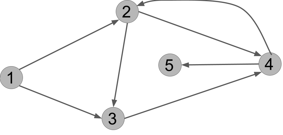
Exercise 8.1 Execute DFS(G,u) on the graph of Figure 7.1, reproduced here. In what order does it print the vertices?

Figure 8.1

Hint: there are multiple correct answers, depending on in which order the neighbors of each vertex are listed.

Example solution.

Here is one answer: u v x y w.

To picture the answer, you can also draw on each vertex the order in which it is marked.

We can also represent the calls to explore() like this:

explore(u)
   explore(v)
      explore(x)
         explore(y)
      explore(w)

This represents the following order of calls to explore. We explore u, which steps to v, which steps to x, which steps to y. At that point, because y has no outgoing edges, the call explore(y) finishes and we backtrack to x. It has another out-edge to v, but v is already marked. So the call explore(x) finishes, and we backtrack to v. It has another out-edge to w, which is not yet marked, so we call explore(w). This call does nothing because w’s only out-neighbor is already marked. Then the call to explore(v) is finally done, and we go back to u. It has another out-neighbor w, but w is already marked by now, so we’re done.

Notes. If the graph is fully connected, then we will eventually call explore() on every vertex. However, if the graph is not connected, then DFS(G) will only explore nodes reachable from \(s\).. You can see this by trying the code on small examples of connected and disconnected graphs.

In many applications, we would replace line 3 of explore(v) with some useful operation involving vertex v. As long as that operation takes constant time, the complexity analysis below will still apply. If not, the analysis below could be modified accordingly.

8.1.1 Search trees

Given a graph, the execution of DFS produces a search tree, which we define as follows. The root is the first vertex \(r\) on which we call explore(r). Then, for each node \(v\), its children are all the nodes \(w\) where we call explore(w) from within the call to explore(v).

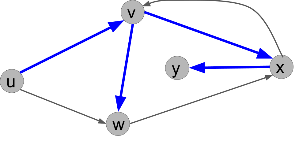
For example, for the sample solution of Exercise 8.1, we get the following search tree (the blue edges), where the root is \(u\).

Figure 8.2

Exercise 8.2 Explain why the following search tree can not be obtained by running DFS(u), no matter what order ties are broken in.

Figure 8.3

Solution.

From u, we either call explore(v) or explore(w) first. If we call explore(v) first, then v would always call explore(w) before u does, so the tree would have to have the edge (v,w) and not the edge (u,w). On the other hand, if we call explore(w) first, then that call would immediately call explore(x) because x would be unmarked. So the edge (w,x) would have to be present in the tree. Either way, the given search tree is not possible.

8.1.2 Runtime analysis

We now analyze the runtime of DFS. This is an interesting problem because it is recursive, but it is not a divide-and-conquer algorithm. We will need to carefully track the resource usage over the course of the algorithm. Recall that \(n\) is the number of vertices in \(G\) and \(m\) is the number of edges.

First, we need to settle on an input representation. We will choose an adjacency list. This implies that we can iterate over the neighbors \(N(v)\) of \(v\) in time \(O(|N(v)|)\), i.e. the number of neighbors. Recall that if we were using an adjacency matrix, then iterating through the neighbors of \(v\) would take \(O(n)\) time regardless of the number of neighbors.

Now we prove some useful facts.

Lemma 8.1 For each vertex \(u\) in the graph, explore(u) is called exactly once.

Proof. Each vertex \(u\) starts unmarked (meaning that marked[u] is False) and is set to marked immediately when explore(u) is called. Since every call to marked(u) is protected by a statement of if not marked[u], explore(u) can only be called once. But the for loop of line 4 of DFS ensures that explore is called for every vertex.

Now, we can analyze the runtime.

Proposition 8.1 DFS runs in time \(O(n + m)\), where \(n\) is the number of vertices and \(m\) is the number of edges.

Proof. The total work can be counted as the work done within DFS(G), which is called once, plus the sum of the work done in all the calls to explore(). We have shown that DFS(G) does \(O(n)\) work internally. We have: \[\begin{align*} \sum_{u \in V} \left(3 |N(u)| + 2 \right) &= 3 \left(\sum_{u \in V} |N(u)|\right) + 2n \\ &= 3 (2m) + 2n \\ &= 6m + 2n . \end{align*}\] We used that the sum of the number of neighbors in the graph is equal to twice the number of edges. Adding this to the \(O(n)\) used by DFS, we get a total running time bound of \(O(n + m)\).

8.1.3 Application: connectivity

DFS has many applications, but here is a simple one. Recall that an undirected graph is connected if there is a path from any vertex to any other vertex. Otherwise, it is disconnected.

Algorithm 8.2 (Connectivity)  

is_connected(G):
   pick any vertex s of G
   DFS(G, s)
   for each vertex v in G:
      if not marked[v]:
         return false
   return true

In alg. 8.2, we simply walk the graph from any starting vertex using DFS. When it returns, we check if every vertex has been marked. If so, we return true (the graph is connected), but if there is an unmarked vertex, we return false.

Exercise 8.3 What is the running time of is_connected(G)?

Solution.

It is \(O(n + m)\), because it calls DFS, which is \(O(n + m)\), and then does \(O(n)\) work itself due to the for loop.

Theorem 8.1 The algorithm is_connected(G) is correct, i.e. returns true if and only if \(G\) is connected.

Proof. First, we have to show it’s correct on any connected graph. If \(G\) is connected, then for every \(v\), there is a path from \(s\) to \(v\). The path looks like \(s, u_1, u_2, \dots, u_k, v\). Well, since there is an edge from \(s\) to \(u_1\), we know that we call explore(u1) at some point. Since there is an edge from \(u_1\) to \(u_2\), we know we call explore(u2) at some point. Repeating, we eventually call explore(v). So \(v\) is marked. This holds for every \(v\), so is_connected(G) will be correct.

Now suppose \(G\) is not connected. Then there are two vertices \(v,w\) with no path between them. That means that \(s\) cannot have a path to both of them, since otherwise there would be a path between them that goes through \(s\). So there is some vertex, call it \(v\), with no path to \(s\). But DFS(G, s) only explores \(s\), vertices with an edge from \(s\), vertices with an edge from those vertices, etc. So it only explores a vertex if there is a path to that vertex from \(s\). So \(v\) is never marked, so is_connected(G) will be correct.

Notice that in the proof, it didn’t matter what vertex \(s\) we started from: the proof works for any \(s\).

8.2 Breadth-first search

Now we’ll look at a different way to explore graphs, breadth-first search (BFS). Unlike DFS, in BFS we first look at all neighbors of the starting node, then all of its neighbors, and so on.

BFS will need a data structure called a queue, more specifically a First-In-First-Out (FIFO) queue. This data structure can be pictured as a list that supports the following operations:

FIFO Queue:

Operation	Time complexity	Meaning
append\((v)\)	\(O(1)\)	add \(v\) to the end of the list
pop\(()\)	\(O(1)\)	remove and return the first item of the list
size\(()\)	\(O(1)\)	return current size of list

This data structure can be implemented e.g. with a linked list. Given a FIFO queue, BFS can be defined as follows:

Algorithm 8.3 (Breadth-First Search)  

BFS(G, s):
   # G = (V,E) is an undirected graph and s a vertex
   for each u in V:
      let marked[v] = False
   let Q = new FIFO_Queue
   Q.append(s)
   set marked[s] = True
   while Q.size() > 0:
      let u = Q.pop()
      print u                  # or do other useful work
      for each neighbor v of u:
         if not marked[v]:
            Q.append(v)
            set marked[v] = True

We can think of BFS as expanding outward in a wave, or in “layers”. The zeroth layer is the start vertex, \(s\). The next layer consists of all neighbors of \(s\). These are all inserted into the queue before any other vertices, so they are popped from the queue before others as well. The next layer are all “neighbors of neighbors”, and so on.

Exercise 8.4 Execute BFS(G,u) on this graph. In what order does it print the vertices?

Figure 8.4

Example solution.

There are multiple solutions depending on the ordering of the vertices, but here is one: \(u, v, w, x, y\). In other words, the vertices are popped from the queue in this order:

Figure 8.5

• First, the start vertex, \(u\), is popped. Its two out-neighbors are \(v\) and \(w\), and both are unmarked. It places them in the queue, let’s suppose in the order \(v,w\).
• Then, \(v\), is popped. Its two out-neighbors are \(x\) and \(w\). First, \(x\) is unmarked, so it is added to the queue. But \(w\) is already marked, so it is not added again.
• Then, \(w\) is popped. Its one out-neighbor is \(x\). But \(x\) is already marked, so nothing happens.
• Then, \(x\) is popped. Its two out-neighbors are \(y\) and \(v\). First, \(y\) is unmarked, so it is added to the queue. But \(v\) is already marked and is not added.
• Finally, \(y\) is popped. It has no out-neighbors.
• Now the queue is empty and the algorithm halts.

In the case of BFS, the search tree consists of edges \((u,v)\) if, when we popped \(u\) from the queue and considered its neighbor \(v\), we called Q.append(v). This represents that we “found” \(v\) from \(u\).

Exercise 8.5 What is a search tree corresponding to BFS(G,u)?

Example solution.

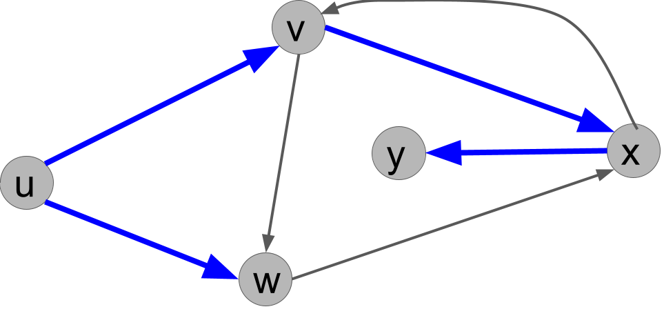
There are multiple correct answers. For the example BFS traversal in the sample solution to Exercise 8.4, the BFS search tree is:

Figure 8.6

8.2.1 Comparing BFS and DFS

With practice, you should be able to run DFS and BFS in your head on small graphs and compare their search trees, as well as all possible search trees that each can produce. Can you solve this exercise?

Exercise 8.6 For the example graph above (Figure 8.4), is there any search tree that can arise from both BFS(G,u) and DFS(G,u)? If so, give it. If not, explain why not.

Solution.

The answer is no. To see why, note that a BFS search tree must contain both \((u,v)\) and \((u,w)\), because the first thing it does is pop \(u\) and add \(v\) and \(w\) (in some order). But we claim no DFS search tree can contain both those edges. To prove that, note the first recursive call is either explore(v) or explore(w). If explore(v), it must eventually called explore(w) from \(v\) before coming back to \(u\), so \((v,w)\) is in the DFS search tree, so \((u,w)\) cannot be: we can’t add \(v\) twice. On the other hand, if the first recursive call is explore(w), then the next call will be explore(x) and from \(x\) we will call explore(v), all before we backtrack to \(u\). So we won’t call explore(v) from \(u\).

8.2.2 Runtime analysis

To analyze BFS, we need to make one observation.

Lemma 8.2 In BFS, every vertex is added to \(Q\) at most once.

Proof. Each place in the code that we add a vertex to \(Q\), namely lines 6 and 13, we immediately set that vertex as marked. And we only ever add unmarked vertices to Q, so each vertex can only be added once.

Theorem 8.2 The runtime of BFS is \(O(n + m)\), where \(n\) is the number of vertices and \(m\) is the number of neighbors.

Proof. We can analyze BFS as follows.

BFS(G, s):
    # G = (V,E) is an undirected graph and s a vertex
    for each v in V:              # O(n) total
       let marked[v] = False      # O(1) each time
    let Q = new FIFO_Queue        # O(1)
    Q.append(s)                   # O(1)
    set marked[s] = True          # O(1)
    while Q.size() > 0:           # at most n iterations
       let v = Q.pop()            # O(1) each time
       print v                    # O(1) each time
       for each neighbor w of v:  # O(|N(v)|) iterations
          if not marked[w]:       # O(1) each time
             Q.append(w)          # O(1) each time
             set marked[w] = True # O(1) each time

As with DFS, the key for the for loop of line 11 is to not consider the worst-case every time. Instead, we add up the total amount of work done by those lines of the algorithm over the course of the algorithm. This total is \(O(\sum_{v \in V} |N(v)|) = O(n + m)\). We also have that lines 8-10 contribute a total of \(O(n)\), and the same for lines 2-7. The total is \(O(n + m)\).