17 Reductions and Applications
This section discusses how we can solve other problems by turning them into max-flow problems.
Objectives. After learning this material, you should be able to:
- Construct reductions from related problems or variants to max flow.
- Identify failures of incorrect reductions.
17.1 Variants of max flow
First, we will look at other versions of the max flow problem. It would be nice if we didn’t have to come up with a new algorithm every time we changed the problem slightly! As we will see, often we can solve a slightly different problem by “reducing” it to max flow.
17.1.1 Antiparallel edges
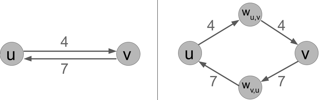
A pair of antiparallel edges are \((u,v)\) and \((v,u)\), i.e. two directed edges between two vertices pointing opposite directions. Remember that we solved max flow assuming that the input graph contains no antiparallel edges.
Actually, one can modify our solution to account for antiparallel edges, but here is a method using a reduction.
- We take as input a flow instance \(G_1, c_1\) that may contain antiparallel edges.
- We use it to construct a new flow instance \(G_2, c_2\) that does not contain any antiparallel edges.
- We run our max flow algorithm, such as Edmonds Karp, on \(G_2, c_2\). It produces some output flow \(f_2\).
- We use \(f_2\) to construct a solution \(f_1\) for the original instance.
Here’s how we construct \(G_2\) and \(c_2\).
- \(G_2\) will contain all of the vertices of \(G_1\), plus more vertices defined below.
- For every edge \((u,v)\) in \(G_1\), we can create a new vertex, call it \(w_{u,v}\). Note that \(w_{u,v}\) is different from \(w_{v,u}\).
- Then, we create two new edges: \((u, w_{u,v})\) and \((w_{u,v},v)\).
- We make the capacity of these new edges equal to the old capacity, i.e. \(c_2(u, w_{u,v}) = c_2(w_{u,v},v) = c_1(u,v)\).
Now, we need to explain how to convert \(f_2\) into \(f_1\).
- For each vertex of the form \(w_{u,v}\), we let \(f_1(u,v) = f_2(u,w_{u,v})\). Note by the net flow constraint, this equals \(f_2(w_{u,v},v)\).
- This defines the flow on every edge of the original graph \(G_1\).
Proposition 17.1 The above reduction is correct, i.e. \(f_1\) is a maximum valid flow for \(G_1, c_1\).
Proof. First, we need to prove that \(G_2\) has no antiparallel edges. That will tell us that \(f_2\) is a correct output for \(G_2, c_2\). Then, we need to prove that, since \(f_2\) is correct, \(f_1\) is correct.
To show \(G_2\) has no antiparallel edges, notice that every edge in \(G_2\) is either of the form \((u, w_{u,v})\) or \((w_{u,v}, v)\). In either case, there is no antiparallel edge. For example, if originally there was an antiparallel edge \((v,u)\), then there will be an edge \((v, w_{v,u})\), but \(w_{v,u}\) is a different vertex than \(w_{u,v}\).
Now, we know \(f_2\) is a max flow for \(G_2, c_2\). Notice that the total amount of flow satisfies \(|f_2| = |f_1|\). So we just need to show that the min \(s-t\) cut the graphs are equal. This will imply that \(f_1\) is a max flow for \(G_1, c_1\). (Actually, we are using the fact that the max-flow min-cut theorem applies for graphs with antiparallel edges, but this turns out to be true.)
Let \(S_1,T_1\) be an \(s-t\) cut in \(G_1, c_1\). The capacity of the cut is \(K(S_1,T_1) = \sum_{u \in S_1,v \in T_1} c(u,v)\). Now consider the following cut in \(G_2, c_2\): We first let \(S_2 = S_1, T_2 = T_1.\) Then, we add all vertices of the form \(w_{u,v}\) to the same element as \(u\). Now, we claim that \(K(S_2,T_2) = K(S_1,T_1)\). This follows because the only edges crossing the cut are of the form \((w_{u,v}, v)\) and they cross the cut if and only if \((u,v)\) crosses the cut \(S_1,T_1\) in the original graph. And they have the same capacity, i.e. \(c_2(w_{u,v},v) = c_1(u,v)\).
17.1.2 Multiple sources and sinks
Suppose we have a max flow problem, but there are multiple possible sources of flow and multiple possible sinks. The new goal is to maximize the total flow into all of the sinks. The constraints on a flow are the same, except that now the net flow constraint does not apply to any of the sources or sinks.
Exercise 17.1 Give a reduction from max flow with multiple sources and sinks to max flow. Sketch a proof of correctness.
Example solution.
First we give the reduction. As before, we need two parts:
- Given an instance \(G_1,c_1\) of the problem of max flow with multiple sources and sinks, construct an instance \(G_2,c_2\) of max flow.
- Given the solution \(f_2\) to max flow, construct the solution \(f_1\) to max flow with multiple sources and sinks.
For 1, Let \(G_1,c_1\) be the original graph. We construct a new graph \(G_2\) by taking a copy of \(G_1\) and adding a “supersource” \(s^*\) and “supersink” \(t^*\). For each source \(s\) in \(G_1\), we add an edge \((s^*, s)\) with capacity infinity. (Actually, we can just set the capacity to any large enough number, e.g. the sum of all the capacities of the original graph.) For each sink \(t\) in \(G_1\), we add an edge \((t, t^*)\) with capacity infinity as well.
For 2, given \(f_2\), we simply remove \(s^*,t^*\) and all of their edges, and this gives us \(f_1\).
Now that we have the reduction, we sketch a proof of correctness. \(G_2,c_2\) is a valid instance of max flow, since it has only one source and one sink. Informally, the reduction works because we allowed it to send as much flow out of each source \(s\) and as much flow into each sink \(t\) as possible, while otherwise respecting all the constraints of a flow. More formally, we again need to know that the max-flow min-cut theorem applies with multiple sources and sinks, which it does (where the cut must have all sources in \(S\) and all sinks in \(T\)). In this case, we can see that a min cut of \(G_2,c_2\) would never contain any of the “infinity” edges, so a min cut in \(G_2,c_2\) is the same as in \(G_1,c_1\). Since the flow amounts are the same as well, this proves that \(f_1\) is optimal in \(G_1,c_1\).
17.2 Bipartite Matching
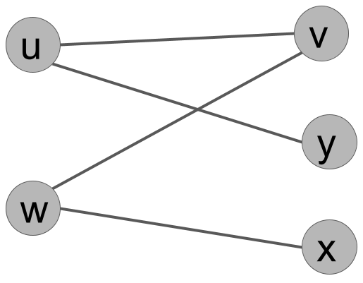
Now we will use max flow to solve a problem that initially seems unrelated. A graph \(G = (V,E)\) is bipartite if the vertices can be partitioned into two sets, \(V_1,V_2\), such that every edge has one endpoint in \(V_1\) and one in \(V_2\).
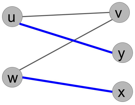
A matching in a graph is a set of edges where no two edges share an endpoint. The size of the matching is the number of edges.
The Maximum Bipartite Matching Problem:
- Input: an undirected bipartite graph \(G\).
- Output: a maximum-sized matching in \(G\).
17.2.1 The reduction
To solve maximum bipartite matching, we will reduce it to max flow.
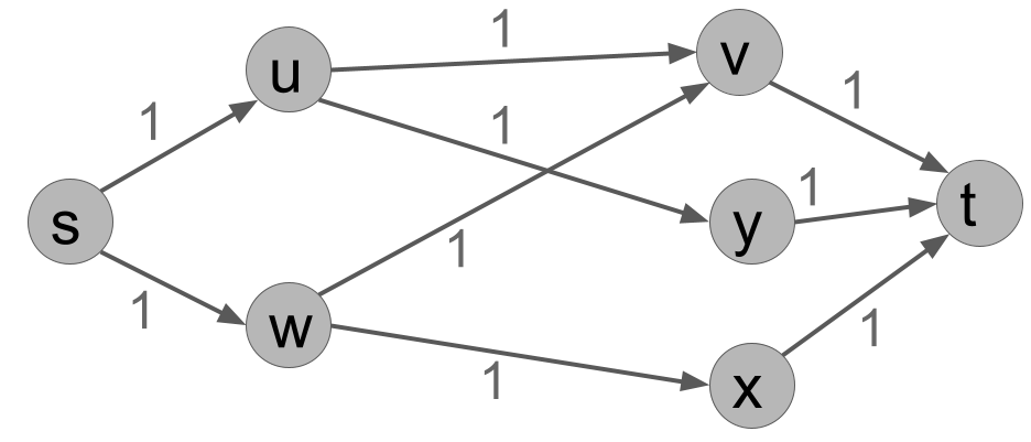
Specifically, let the input be \(G = (V,E)\) with \(V\) partitioned into \(V_1,V_2\). We create a new graph \(G' = (V',E')\) and capacity \(c'\) as follows.
- Start with a copy \(V'\) of all the vertices \(V\).
- For every edge of the form \(\{u,v\} \in E\), where \(u \in V_1\) and \(v \in V_2\), create a directed edge \((u,v) \in E'\) and set \(c(u,v) = 1\).
- Create a new vertex \(s \in E'\), the source.
- Create an edge \((s,u)\) for every \(u \in V_1\), setting \(c(s,u) = 1\).
- Create a new vertex \(t \in E'\), the source.
- Create an edge \((v,t)\) for every \(v \in V_2\), setting \(c(v,t) = 1\).
We then solve max flow on \(G',c'\) obtaining a flow \(f'\). Given \(f'\), we convert it to a matching as follows:
- For each edge \(\{u,v\}\) of the original graph, if \(f'(u,v) > 0\), then we add \(\{u,v\}\) to our matching.
17.2.2 Correctness and the Integrality Theorem
It turns out that this reduction is not always correct unless we use the right kind of max flow algorithm. Can you find the problem?
Exercise 17.2 For the example graph above (Figure 17.1, Figure 17.2), give an example flow \(f'\) that is a max flow in the reduction graph \(G',c'\), but does not yield a valid matching.
Hint: your flow amounts should not all be integers on all edges.
Example solution.
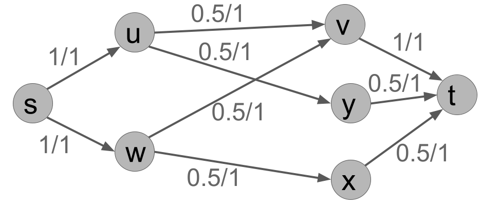
According to the reduction, we would try to add all four middle edges, which would not yield a valid matching (the endpoints \(u\), \(w\), and \(v\) are all included twice).
Luckily, however, our reduction will be correct when using Ford-Fulkerson algorithms. Specifically, we will need to find a max flow where the flow amounts are 0 or 1. Luckily, when the input capacities are all 0 or 1, then so are the output flows – if we use a Ford-Fulkerson algorithm. This is a consequence of the following theorem.
Theorem 17.1 (The Integrality Theorem) A max-flow instance where all capacities are integers always has a solution where all flows are integers. Morever, any Ford-Fulkerson algorithm always finds an all-integer max flow.
Proof. At the beginning of the algorithm, all residual capacities are integers, because the capacities are integers and the flow is zero everywhere. So regardless of what augmenting path is chosen, the augmentation amount is an integer.
Therefore, after the first step, the flow on every edge is an integer (either zero or the augmentation amount), and the capacities are always integers, so the residual capacities are still integers. So regardless of the augmenting path, the augmentation amount is an integer.
Continuing the argument, at every stage of the algorithm, the flow amount on every edge is always an integer, including when the algorithm halts. We also see that any Ford-Fulkerson algorithm must halt here, because every augmentation amount is at least 1, and we can only augment by 1 a finite number of times until we reach the max flow.)
We know that, when a FF algorithm halts, it must have found a max flow. Since we know the FF algorithm halts with an all-integer flow, we also conclude that an all-integer max flow must exist.
Proposition 17.2 When using a Ford-Fulkerson algorithm for max flow, our reduction is correct (i.e. we output a maximum matching).
Proof. By the Integrality Theorem, all flows are integers. Since the capacities are all 1, this means every edge’s flow is either zero or one.
Consider a vertex \(u \in V_1\). It has exactly one incoming edge (from \(s\)). So the maximum amount of flow through \(u\) is 1. Because the flows are integers, this means that at most one edge out of \(u\) has flow 1. So at most one edge incident to \(u\) is in the matching.
Similarly, for any \(v \in V_2\), it has exactly one outgoing edge (to \(t\)), so at most one edge incident to \(v\) is in the matching.
This proves that the matching we output is indeed a valid matching, i.e. it does not include more than one edge incident to any vertex. Furthermore, we note that the number of edges in the matching is exactly equal to the amount of flow. Now we need to prove that we output the maximum matching.
To do so, consider any valid matching in the graph. We can turn it into a valid flow in our flow graph: for every edge \(\{u,v\}\) in the matching with \(u \in V_1, v \in V_2\), we send one unit of flow along \((s,u)\), one along \((u,v)\) and one along \((v,t)\). All of the capacity and flow constraints are satisfied because every \(u\) and \(v\) are only in the matching at most once. Furthermore, the amount of flow is exactly the number of edges in the matching.
Because every valid matching corresponds to a flow graph with the same amount of flow and vice versa, the maximum matching corresponds to the maximum flow.