7  Graphs and Trees

This section introduces graphs and graph terminology. Many, many computational problems are modeled as problems to do with graphs, as we will soon see.

Objectives. After learning this material, you should be able to:

• Recall and apply definitions such as graph, neighbors, degree, paths, etc.
• Constrast the performance of the adjacency matrix and the adjacency list representations of a graph.
• Recall and apply definitions for trees, including root, children, height, etc.

7.1 Graphs, formally

As you know, graphs represent a set of objects (the vertices) and relationships between the objects (the edges). Grahps are used to model many settings, such as:

• Road networks
• Computer networks
• Social networks (friendship graphs)
• Web pages and hyperlinks
• Financial networks
• Biological systems
• States of a system and transitions between states

Formally:

Definition 7.1 (Graph) A graph \(G = (V,E)\) consists of a set of vertices (also called nodes), \(V\), and a set of edges, \(E\). The graph is directed if each edge \(e = (u,v)\) represents an ordered pair, where the edge goes from \(u\) to \(v\). The graph is undirected if each edge \(e = \{u,v\}\) represents an unordered pair, where the edge equally connects \(u\) to \(v\) and \(v\) to \(u\).

The number of vertices is \(|V|\) and is usually called \(n\). The number of edges is \(|E|\) and is usually called \(m\).

For example, in a social network, the vertices are people, and there is an edge \((u,v)\) if person \(u\) is “following” person \(v\). We also recall these useful graph concepts.

• A neighbor of \(u\) in an undirected graph is a vertex \(v\) with whom \(u\) shares an edge. We sometimes use \(N(u)\) to denote the set of neighbors of \(u\).
  • The degree of \(u\) in an undirected graph is the number of its neighbors.
• An out-neighbor of \(u\) in a directed graph is a \(v\) for which \((u,v)\) is an edge. Similarly, an in-neighbor is a \(v\) for which \((v,u)\) is an edge.
  • The out-degree is the number of out-neighbors; similarly for in-degree.
• A path in a graph is a list of vertices \(v_1,\dots,v_k\) where there is an edge from each vertex to the next. In a directed graph, the edges must “point” forward. The length of the path is the number of edges, i.e. \(k-1\).
• A cycle in a graph is a path \(v_1,\dots,v_k\) of length at least \(2\) where \(v_k = v_1\), i.e. we end where we started.
  • Often, when we say cycle, we really mean simple cycle, which is a cycle that does not have any repeated edges or vertices. It is always good to double-check whether simple cycle is meant.

Test your understanding of the terminology:

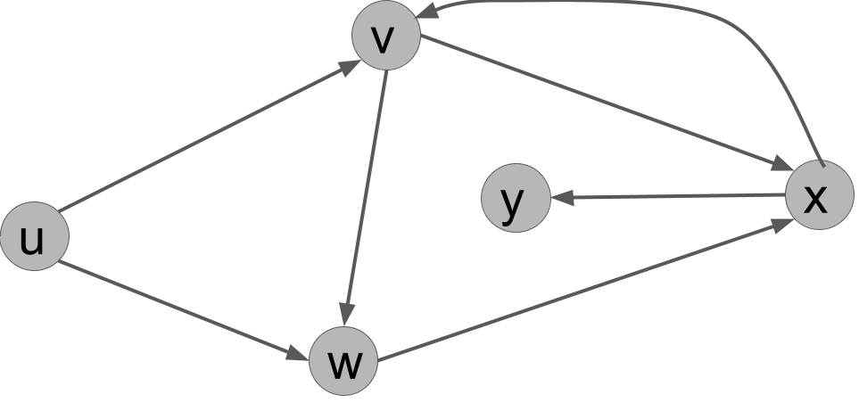
Exercise 7.1 For the following directed graph (Figure 7.1), answer these questions:

1. List all the edges in the graph.
2. What is the out-degree of \(u\)?
3. Name all of the in-neighbors of \(v\).
4. Is \((u,v,w,x,y)\) a path in the graph?
5. Is \((u,w,y,x,v)\) a path in the graph?
6. What is a cycle in the graph?

Figure 7.1

Solutions.

1. \((u,v), (u,w), (v,w), (v,x), (w,x), (x,v), (x,y)\).
2. \(2\).
3. \(u\) and \(x\).
4. Yes.
5. No: there is no edge from \(y\) to \(x\).
6. There are several answers. One cycle is \(v,w,x,v\). This is a cycle because it is a path (a list of vertices where an edge connects each vertex to the next) and the last vertex in the list equals the first.

Here is a fun fact that will be useful later:

Proposition 7.1 In an undirected graph, the sum of the degrees of the vertices is equal to twice the number of edges.

Proof. Every edge has two endpoints, e.g. \(u\) and \(v\). If we sum over the vertices the degree of each vertex, then for \(u\), the edge is counted once, and for \(v\), the edge is counted once. Therefore, each edge is counted twice in total.

7.1.1 Adjacency matrix representation

How do we write a graph down for a computer to work with? There are two main ways. The first is called the adjacency matrix representation. For a graph with \(n\) vertices, it is an \(n \times n\) matrix, where a \(1\) in the \((u,v)\) entry represents that there is a directed edge from \(u\) to \(v\). If the graph is undirected, then the matrix is symmetric, i.e. there is \(1\) at position \((u,v)\) if and only if there is a \(1\) at position \((v,u)\).

Example 7.1 For the example graph above (Figure 7.1), here is its adjacency matrix:

	u	v	w	x	y
u	0	1	1	0	0
v	0	0	1	1	0
w	0	0	0	1	0
x	0	1	0	0	1
y	0	0	0	0	0

The adjacency matrix data structure has the following important characteristics:

• Space: the size of the data structure is \(n^2\) regardless of the number of edges.
• Edge query: checking whether an edge \((u,v)\) exists or not is an \(O(1)\) time operation. We can just jump to the appropriate location in the list and check.
• Neighbors query: getting the list of out-neighbors of a vertex \(u\) is an \(O(n)\) time operation, because we need to scan the entire \(u\) row of the matrix to check for all the neighbors.

7.1.2 Adjacency list representation

The second main way to write down a graph is as an adjacency list. This consists of an array of lists. For each vertex, we give a list of its out-neighbors.

For the example graph above (Figure 7.1), here is its adjacency list:

vertex	out-neighbors
u	v, w
v	w, x
w	x
x	v, y
y

The adjacency list data structure has the following characteristics:

• Space: the size of the data structure is \(O(n + m)\), where \(n\) is the number of vertices and \(m\) is the number of edges.
• Edge query: checking whether an edge \((u,v)\) exists is no longer constant time, but involves scanning through the list associated with \(u\) for the presence of \(v\).
• Neighbors query: getting the list of out-neighbors of a vertex is now \(O(1)\) time, because it is already written down for us.

We can see that the adjacency list might be much smaller to store than the adjacency matrix and can be faster if we need to iterate through the neighbors of vertices. However, the adjacency matrix is faster for looking up existence of given edges.

7.1.3 Weighted graphs

A weighted graph is a graph where, for each edge \((u,v)\), we are given a weight \(w(u,v) \in \mathbb{R}\). The graph can be either directed or undirected.

With adjacency matrices, we can represent the weight directly in the entry of the matrix, replacing \(1\) with the actual weight. Depending on the application, we may treat a weight of zero or a weight of infinity as “edge does not exist”. With adjancency lists, we can simply store the weights in the lists next to the corresponding neighbor.

In a weighted graph, the length of a path is now the sum of the weights along the path. Here is an example weighted graph:

Figure 7.2

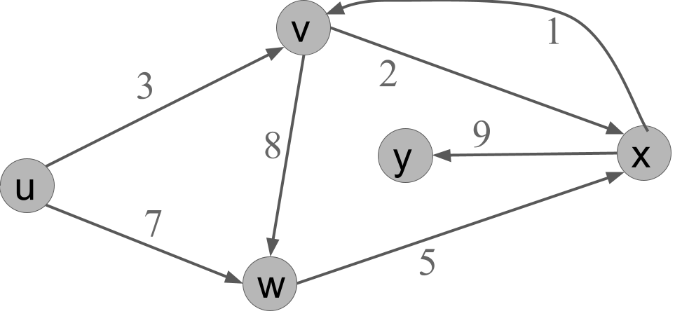
In this graph, the path \(u,v,w,x\) has length \(3 + 8 + 5 = 16\).

7.2 Trees

A tree is a special type of graph. We will define trees inductively.

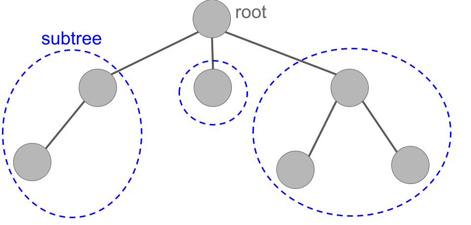
Definition 7.2 (Tree) A tree is a graph organized as follows. There is a vertex \(r\) called the root.

• \(r\) by itself with no edges is a tree.
• Given a set of trees \(T_1,\dots,T_k\) with roots \(v_1,\dots,v_k\) respectively, the graph produced by connecting \(r\) to each of \(v_1,\dots,v_k\) is a tree. In this case, we say \(r\) is the parent of each \(v_i\), which is a child of \(r\).

Technically, this is called a rooted tree. If we form a rooted tree, then take away the designation of which node is the root node, we are left with a regular old tree. We will come back to those later in the course, but focus on rooted trees for now.

Figure 7.3

Let us practice induction by proving an important fact.

Theorem 7.1 A tree with \(n\) vertices always has \(n-1\) edges.

Proof. The base case is a tree with \(n=1\) vertex, which has \(0=n-1\) edges as required.

For the inductive case, let \(n \geq 2\) and suppose all trees with \(t < n\) vertices have \(t-1\) edges. A tree on \(n\) vertices is formed by a root \(r\) connected to a set of trees \(T_1,\dots,T_k\). These have a total of \(n-1\) vertices, since adding the root makes \(n\). Therefore, they have a total of \(n-1-k\) edges, because each tree contributes one fewer edges than vertices by inductive hypothesis. Now we need to add the edges between \(r\) and the roots of each of the subtrees, which adds \(k\) edges. The total is \(n-1\).

We recall some more tree terminology:

• A vertex with no children is called a leaf.
• The height of a tree is the length of the longest path from the root to a leaf.
• An ancestor of a vertex is a parent, parent of a parent, etc. all the way back up to the root.
• A descendent of a vertex is a child, child of a child, etc.